![]()
![]()
![]()
Use LEFT and RIGHT arrow keys to navigate between flashcards;
Use UP and DOWN arrow keys to flip the card;
H to show hint;
A reads text to speech;
37 Cards in this Set
- Front
- Back
|
Correlation formula |
p1,2 = Cov1,2 ------------- σ1 σ2 |
|
|
Variance of a two asset portfolio |
with covariance: σ2 = w1^2 *σ1^2 + w2^2*σ2^2 + 2*w1*w2*covariance(1,2)
with correlation: σ2 = w1^2 *σ1^2 + w2^2*σ2^2 + 2*w1*w2*p1,2σ1σ2 |
|
|
Expected return on a 2 asset portfolio |
E(Rp) = w1E(R1) + w2E(R2)
where E(Rp) is the expected return on portfolio P w = weighting of that asset E(R) expected return on that asset
|
|
|
Capital allocation line (CAL) |
describes the combinations of expected return and standard deviation of return available by combining an optimal portfolio of risky assets with the risk-free asset; the graph of this starts at the intersection of the RFR return and is tangent to the efficient frontier of risky assets – the line itself represents an optimal portfolio of risky assets
Y = a +bX E(Rc) = [E(Rt) - Rfr] RfR + --------------------- x σc σt
|
|
|
Capital market line (CML) |
when investors share identical expectations about mean returns, variance of returns, and correlations of risky assets; when the CAL is the same for all investors E(RA) = [E(RM) - Rfr] x σA RfR + --------------- σM
|
|
|
Relationship between CAL and CML |
CML is when the CAL is the same for all investors |
|
|
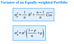
Equally weighted portfolio risk |
|
|
|
CML and CAPM |
CML represents the efficient frontier when the assumptions of the CAPM hold |
|
|
Security market line (SML) |
is the graph of the CAPM model, or the CAPM equation
CAPM = E(Ri) = RFR + Beta * (E(R of Market) – RFR) |
|
|
Beta definition as it relates to the market |
Beta is a measure of the asset’s sensitivity to movements in the market Covi,m ---------- σm^2 σi pi,m x --------- σm pi,mσiσm ------------- σm^2 |
|
|
Market risk premium |
E(Rm) - RFR |
|
|
Sharpe Ratio |
the ratio of mean return in excess of the RFR to the standard deviation of return (E(Ri) – RFR) -------------------- sd of Asset i |
|
|
Adding assets to the portfolio and the Sharpe Ratio |
Adding a new asset to your portfolio is optimal if the following condition holds: |
|
|
Market Model |
describes a regression relationship between the returns on an asset and the returns on the market portfolio |
|
|
Market Model assumptions |
The expected value of the error term is 0 |
|
|
Adjusted beta |
if historical beta is not deemed to be the best predictor, can use adjusted beta |
|
|
Historical beta |
assumes that beta for each stock is a random walk from one period to the next, and the error term mean is “0” – so Beta t+1 = Beta t + error (or 0) |
|
|
Multi-factor model |
multi-factor models could also address: interest rate movements, inflation, or industry-specific returns |
|
|
Active return |
return on portfolio – return on the benchmark (comparable to the portfolio) |
|
|
Active risk |
the standard deviation of active returns |
|
|
Active factor risk |
the contribution to active risk squared resulting from the portfolio’s different-than-benchmark exposures relative to factors specified in the risk model |
|
|
Active selection risk or Active specific risk |
the contribution to active risk square resulting from the portfolio’s active weights on individual assets as those weights interact with assets’ residual risk = sum of weight differences and variances of the asset’s returns unexplained by factors |
|
|
Tracking error |
synonym with active risk, but the term “error” is confusing as it is meant to represent “difference” here |
|
|
Tracking risk |
also a synonym of active risk = |
|
|
Separation theorem |
everyone holds the same portfolio of risky assets and individual investor’s determine the weight of that portfolio with their domestic RFR “separately” |
|
|
Real exchange rate movements |
are defined as movements in the exchange rates that are not explained by the inflation differential between the two countries |
|
|
Foreign currency risk premium working in concert with interest rate parity |
E(R) – RFR, or the expected movement in the exchange rate less the interest rate differential (domestic RFR – foreign RFR), and after factoring in appreciation/depreciation for the period |
|
|
Information ratio |
a tool for evaluating mean active returns per unit of active risk --------------------------------------- = ------ annualized residual risk w
IR = IC x √BR |
|
|
Information Coefficient |
measures managers forecasting accuracy if a manager makes N bets on the direction of the market and Nc are correct, the IC is the covariance between forecast and actual direction of the market
IC = 2x (Ncorrect/Ntotal guesses) - 1
when we add another source of information that is correlated, the skill (IC) of the manager does not increase proportionately. ICcom represents the new info. ICcom = ICorig x √(2/1+r)
where r = correlation
|
|
|
ex-post information ratio |
related to the t-stat one obtains for alpha in the regression of portfolio excess returns against benchmark excess returns: tα t statistic of alpha ---------------------------------------- √n number of years of data |
|
|
Value added |
Objective of active management is to maximize value added
VA = α - (λ x ω^2)
λ = risk aversion ω = residual risk |
|
|
Highest achievable value added * |
function of optimal level of residual risk and the portfolio managers IR
VA* = ω* x IR ---------- or 2
VA* = IR^2 ---------- or 4λ
VA* = IC^2 x√BR ------------- 4λ |
|
|
Breadth |
# of forecasts made in a year
IR = IC x √BR |
|
|
Optimal level of residual risk
ω* |
ω* = IR IC x √BR ----- = ------------ 2λ 2λ
λ = risk aversion |
|
|
Systematic Risk |
reflects factors that have general effect on the securities market as a whole and cannot be diversified away
for example macroeconomic risk represented by Beta |
|
|
Unsystematic risk |
can be reduced through diversification |
|
|
The single factor market model covariance calculation |
One of the predictions of the single-factor market model is that Cov(Ri,Rj) = bibjsM2. In other words, the covariance between two assets is related to the betas of the two assets and the variance of the market portfolio. |